科学计算库
NumPy
记录 NumPy 库的基本用法和常见问题的解决策略。
np.array 用法
使用 np.array() 方法可以使用列表或元组用来初始化一个 numpy 数组,数据类型为 np.ndarray,当然可以通过 dtype 指定元素类型。对于数据类型为 ndarray 的对象 arr,常用的方法包括但不限于以下几种:
创建和初始化
np.array(object, dtype=None):从列表、元组等对象创建一个 ndarray。np.zeros(shape, dtype=float):创建一个全零的数组。np.ones(shape, dtype=float):创建一个全一的数组。np.empty(shape, dtype=float):创建一个未初始化的数组。np.random.rand(shape):返回一个 \([0,1)\) 取值范围的数组。np.arange(start, stop, step, dtype=None):创建一个等差数列的数组。np.linspace(start, stop, num=50, dtype=None):创建一个等间隔的数组。
形状操作
arr.shape:返回数组的形状维度。arr.reshape(newshape):返回改变形状后的数组(注:新形状的元素个数与原来的元素个数必须相等)。arr.flatten():返回将原数组展平后的一维数组。arr.transpose() 或 arr.T:返回转置后的数组。
索引和切片
arr[index]:通过索引访问数组元素。arr[start:stop:step]:通过切片访问数组元素。arr[x, y]:高维元素可以用逗号分隔符访问(注:其中的 x 可以是数字、切片或数组)。
数学运算
axis 是轴的意思,numpy 中 axis=0 表示按列,axis=1 表示按行。
arr.sum(axis=None):计算数组元素的和。arr.mean(axis=None):计算数组元素的平均值。arr.std(axis=None):计算数组元素的标准差。arr.var(axis=None):计算数组元素的方差。arr.max(axis=None):返回数组的最大值。arr.min(axis=None):返回数组的最小值。arr.cumsum(axis=None):返回数组的前缀和。arr.cumprod(axis=None):返回数组的前缀积。
逻辑运算
arr.all():检查数组中所有元素是否为真。arr.any():检查数组中是否有任何元素为真。
排序和搜索
np.sort(arr):返回对数组进行排序的新数组。np.argsort(arr):返回排序后每个位置在原数组中的位置索引。np.argmax(arr):返回数组中最大值的索引。np.argmin(arr):返回数组中最小值的索引。
其他常用方法
arr.astype(dtype):将数组转换为指定数据类型。arr.copy():创建数组的副本。arr.tolist():将数组转换为列表。
矩阵运算
numpy 的矩阵运算没有 matlab 来的那么显然,因为有一些隐式的规则。需要注意的是所有的容器类型全都是 np.ndarray。共分为以下几种数据结构:
标量(Scalar):一个单独的数字,没有维度
向量(Vector):一维数组
矩阵(Matrix):二维数组
张量(Tensor):三维或更多维度的数组
元素级运算
+, -, *, /, ^, sqrt 等和 标量 进行运算时都是元素级运算。和 形状相同 的数组进行运算时也都是元素级运算。例如:
# 输入
a = np . array ([[ 1 , 2 , 3 ],
[ 4 , 5 , 6 ]])
b = np . array ([[ 7 , 8 , 9 ],
[ 10 , 11 , 12 ]])
print ( a + 1 )
print ( a - 2 )
print ( a * b )
print ( a / b )
""" 输出
[[2 3 4]
[5 6 7]]
[[-1 0 1]
[ 2 3 4]]
[[ 7 16 27]
[40 55 72]]
[[0.14285714 0.25 0.33333333]
[0.4 0.45454545 0.5 ]]
"""
若形状不同,则会报错:
ValueError : operands could not be broadcast together with shapes (2, 3) (3, 3)
向量级运算
分为两类:内积(点积)和外积(叉积)
内积相当于 \(A_{1\times n}\times B_{n\times 1}=x\)
外积相当于 \(A_{n\times 1} \times B_{1\times m}=C_{n\times m}\)
内积(点积) 。常用 @ 运算符、np.dot(a, b) 和 a.dot(b) 方法。运算结果为标量。此时可以理解为矩阵运算,但是由于 numpy 的广播机制,我们并不需要保证对齐为 \(1\times n,n\times 1\) 即可自动进行正确运算。例如:
# 输入
a = np . array ([ 1 , 2 , 3 ])
b = np . array ([ 7 , 8 , 9 ])
c1 = a @ b
c2 = np . dot ( a , b )
c3 = a . dot ( b )
print ( c1 , type ( c1 ))
print ( c2 , type ( c2 ))
print ( c3 , type ( c3 ))
""" 输出
50 <class 'numpy.int64'>
50 <class 'numpy.int64'>
50 <class 'numpy.int64'>
"""
注:两向量长度必须完全一致,否则报「矩阵没有对齐」的错误:
ValueError : matmul : Input operand 1 has a mismatch in its core dimension 0, with gufunc signature (n ?, k ), (k , m ?)->(n ?, m ?) (size 3 is different from 4)
外积(叉积) 。常用 np.outer(a, b) 方法。运算结果为矩阵。例如:
# 输入
a = np . array ([ 1 , 2 , 3 , 3 ])
b = np . array ([ 7 , 8 , 9 ])
c = np . outer ( a , b )
print ( type ( c ))
print ( c )
""" 输出
<class 'numpy.ndarray'>
[[ 7 8 9]
[14 16 18]
[21 24 27]
[21 24 27]]
"""
进阶 。如果参与运算的不是向量,而是二维矩阵甚至高维张量,该方法会将非向量数据「展开成向量」进行运算。例如:
# 输入
a = np . array ([[[[[ 1 , 2 ]]], [[[ 3 , 4 ]]], [[[ 5 , 6 ]]]], [[[[ 7 , 8 ]]], [[[ 9 , 1 ]]], [[[ 2 , 3 ]]]]])
b = np . array ([[ 3 , 4 , 5 ], [ 1 , 1 , 1 ]])
c = np . outer ( a , b )
print ( type ( c ))
print ( a . shape )
print ( b . shape )
print ( c . shape )
print ( c )
"""输出
<class 'numpy.ndarray'>
(2, 3, 1, 1, 2)
(2, 3)
(12, 6)
[[ 3 4 5 1 1 1]
[ 6 8 10 2 2 2]
[ 9 12 15 3 3 3]
[12 16 20 4 4 4]
[15 20 25 5 5 5]
[18 24 30 6 6 6]
[21 28 35 7 7 7]
[24 32 40 8 8 8]
[27 36 45 9 9 9]
[ 3 4 5 1 1 1]
[ 6 8 10 2 2 2]
[ 9 12 15 3 3 3]]
"""
矩阵级运算
常用 @ 运算符、np.dot(a, b) 和 a.dot(b) 方法。运算结果为矩阵。
# 输入
a = np . array ([[ 1 , 2 , 3 ],
[ 4 , 5 , 6 ]])
b = np . array ([[ 7 , 8 , 9 ],
[ 10 , 11 , 12 ]])
c1 = a @ b . T
c2 = np . dot ( a , b . T )
print ( a . shape , b . shape , c1 . shape , c2 . shape )
print ( c1 )
print ( c2 )
"""输出
(2, 3) (2, 3) (2, 2) (2, 2)
[[ 50 68]
[122 167]]
[[ 50 68]
[122 167]]
"""
注意:
全都是矩阵。此时与向量自动对齐不同,矩阵运算需要我们手动进行对齐,否则报「矩阵没有对齐」的错误;
既有矩阵也有向量。此时同样需要我们手动对齐,否则报「矩阵没有对齐」的错误。
矩阵运算小结
我们可以将上述总结为「元素级」运算和「矩阵级」运算。向量和矩阵统称为矩阵。张量运算机制暂时不予讨论
对于元素级运算。如果矩阵直接和标量运算就没有约束;如果和另外一个矩阵进行标量运算就需要保证两个矩阵的 形状完全一致 ;
对于矩阵级运算。如果 只有向量 参与运算则无需对齐;如果 存在矩阵 参与运算则必须手动对齐。并且此时 @ 运算符和 np.dot(a, b) 以及 a.dot(b) 完全相同。
Pandas
记录 Pandas 库的基本用法和常见问题的解决策略。Pandas 的基本数据结构由 DataFrame 和 Series 组成,这也是 Pandas 的核心所在。
DataFrame
二维表格型数据结构,带行索引和列标签,是 Pandas 的核心对象。
import pandas as pd
df = pd . DataFrame ({
"int_col" : [ 1 , 2 , 3 , 4 , 5 ],
"text_col" : [ "alpha" , "beta" , "gamma" , "delta" , "epsilon" ],
"float_col" : [ 0.0 , 0.25 , 0.5 , 0.75 , 1.0 ]
})
df.info()。查看数据表基本信息(行数、列数、非空值、数据类型):
import pandas as pd
int_values = [ 1 , 2 , 3 , 4 , 5 ]
text_values = [ 'alpha' , 'beta' , 'gamma' , 'delta' , 'epsilon' ]
float_values = [ 0.0 , 0.25 , 0.5 , 0.75 , 1.0 ]
df = pd . DataFrame ({
"int_col" : int_values ,
"text_col" : text_values ,
"float_col" : float_values
})
df . info ()
""" 输出
<class 'pandas.core.frame.DataFrame'>
RangeIndex: 5 entries, 0 to 4
Data columns (total 3 columns):
# Column Non-Null Count Dtype
--- ------ -------------- -----
0 int_col 5 non-null int64
1 text_col 5 non-null object
2 float_col 5 non-null float64
dtypes: float64(1), int64(1), object(1)
memory usage: 252.0+ bytes
"""
df.describe(include='all')。查看数值型与分类型列的统计特征:
import pandas as pd
int_values = [ 1 , 2 , 3 , 4 , 5 ]
text_values = [ 'alpha' , 'beta' , 'gamma' , 'delta' , 'epsilon' ]
float_values = [ 0.0 , 0.25 , 0.5 , 0.75 , 1.0 ]
df = pd . DataFrame ({
"int_col" : int_values ,
"text_col" : text_values ,
"float_col" : float_values
})
df . describe ( include = 'all' )
""" 输出
int_col text_col float_col
count 5.000000 5 5.000000
unique NaN 5 NaN
top NaN alpha NaN
freq NaN 1 NaN
mean 3.000000 NaN 0.500000
std 1.581139 NaN 0.395285
min 1.000000 NaN 0.000000
25% 2.000000 NaN 0.250000
50% 3.000000 NaN 0.500000
75% 4.000000 NaN 0.750000
max 5.000000 NaN 1.000000
"""
Series
一维带标签数组,常用来表示单列。
s = pd . Series ([ 10 , 20 , 30 ], index = [ "a" , "b" , "c" ])
print ( s [ "a" ]) # 10
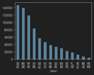
se.plot()。绘制直方图:
plt . figure ( figsize = ( 4 , 3 ))
train [ 'label' ] . value_counts () . plot ( kind = 'bar' )
plt . show ()
文件操作
读:
train_df = pd . read_table ( "train.txt" , sep = " \t " , header = None )
dev_df = pd . read_table ( "dev.txt" , sep = " \t " , header = None )
test_df = pd . read_table ( "test.txt" , sep = " \t " , header = None )
header 参数:表头所在行。例如 header=0。当 header=None 时表示没有表头或不加载表头;
sep 参数:即 separate,表示分隔符。
添加列名:
train_df . columns = [ "feature" , "label" ]
dev_df . columns = [ "feature" , "label" ]
test_df . columns = [ "feature" ]
写:
train_df . to_csv ( "train.csv" , sep = " \t " , index = False )
dev_df . to_csv ( "dev.csv" , sep = " \t " , index = False )
test_df . to_csv ( "test.csv" , sep = " \t " , index = False )
数据处理
索引 。分以下四种:
loc:行号、列标签,能切片;iloc:行号、列号,能切片;at:单个元素(行号 + 列标签),更快;iat:单个元素(行号 + 列号),更快。
如下示例:
locilocatiat
# 准备数据
df = pd . DataFrame ({
"name" : [ "Alice" , "Bob" , "Charlie" ],
"age" : [ 23 , 30 , 27 ],
"score" : [ 85 , 92 , 78 ]
})
# 单个元素
print ( df . loc [ 0 , "age" ])
"""
23
"""
# 多行多列
print ( df . loc [ 0 : 1 , [ "name" , "score" ]])
"""
name score
0 Alice 85
1 Bob 92
"""
# 准备数据
df = pd . DataFrame ({
"name" : [ "Alice" , "Bob" , "Charlie" ],
"age" : [ 23 , 30 , 27 ],
"score" : [ 85 , 92 , 78 ]
})
# 单个元素
print ( df . iloc [ 0 , 1 ])
"""
23
"""
# 多行多列
print ( df . iloc [ 0 : 2 , [ 0 , 2 ]])
"""
name score
0 Alice 85
1 Bob 92
"""
# 准备数据
df = pd . DataFrame ({
"name" : [ "Alice" , "Bob" , "Charlie" ],
"age" : [ 23 , 30 , 27 ],
"score" : [ 85 , 92 , 78 ]
})
# 单个元素(比 loc 更快)
print ( df . at [ 0 , "age" ])
"""
23
"""
# 准备数据
df = pd . DataFrame ({
"name" : [ "Alice" , "Bob" , "Charlie" ],
"age" : [ 23 , 30 , 27 ],
"score" : [ 85 , 92 , 78 ]
})
# 单个元素(比 iloc 更快)
print ( df . iat [ 0 , 1 ])
"""
23
"""
拷贝 。如下示例:
test_copy = test_df . copy ( deep = True )
添加新列 。如下示例:
test_copy [ "label" ] = "unknown"
布尔索引 。如下示例:
# 统计某个条件的数量
unknown_count = ( test_copy [ "label" ] == "unknown" ) . sum ()
# 筛选数据
filtered_df = test_copy [ test_copy [ "label" ] != "unknown" ]
统计转换
按行合并:
merged_df = pd . concat ([ train_df , test_copy ], axis = 0 )
按行遍历:
这个问题很有代表性:Pandas 按行遍历是很多人第一直觉,但其实在性能上是“不得已而为之”的手段,因为 Pandas 更推荐向量化运算或 apply。完整地说,常见写法有以下几类:
iterrows(),最常见的写法。逐行返回 (index, Series),使用起来直观,但慢,尤其是大数据量:
for idx , row in df . iterrows ():
print ( idx , row [ "int_col" ], row [ "text_col" ])
缺点:返回的是 Series,数据类型可能被强制转换(int → float)。
itertuples(),更快的方式。逐行返回 namedtuple,访问列时用属性(点操作符),速度比 iterrows() 快得多:
for row in df . itertuples ( index = True , name = "Row" ):
print ( row . Index , row . int_col , row . text_col )
注意:默认 index=True,会把索引当作第一个字段;name=None 时返回普通 tuple,更快但可读性差。
apply(),用函数“按行处理”。apply(func, axis=1) 可以让你写一个函数处理每一行,返回新的 Series 或 DataFrame:
df [ "new_col" ] = df . apply ( lambda row : row [ "a" ] + row [ "b" ], axis = 1 )
适合“逐行生成新列”的情况。
向量化(推荐优先)。很多场景根本不需要逐行遍历,直接用列运算更高效:
df [ "new_col" ] = df [ "a" ] + df [ "b" ]
这其实等价于上面 apply 的效果,但性能要好得多。
Matplotlib
记录 Matplotlib 库的基本用法和常见问题的解决策略。
解决中文显示异常问题
最简单的方法就是直接在全局区加下面四行代码:
import matplotlib.pyplot as plt
import matplotlib as mpl
mpl . rcParams [ 'font.family' ] = 'SimHei'
plt . rcParams [ 'axes.unicode_minus' ] = False
更详尽的方法可以参考 Matplotlib 中正确显示中文的四种方式 这篇博客。
2025年9月11日
2024年6月20日
GitHub